Sutton Book Notes
Chapter 3: Finite Markov Decision Processes
Problem Formulation: “an agent learns from interaction (with environment) to achieve a goal”.
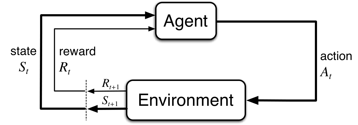
At each time step $t$:
- Agent gets a state $S_t$ from environment.
- Agent selects an action $A_t$ based on $S_t$.
- Agent receives a reward $R_{t+1}$ from environment, and finds itself in a new state $S_{t+1}$.
At each time step $t$, the agent implements a mapping from states to probabilities of selecting each possible action, called policy, denoted $\pi_t$. $\pi_t(a|s)$ is the probability that $A_t = a$ if $S_t = s$.
The agent’s goal is to maximize the cumulative reward it receives over the long run, often called return: $$ G_t = \sum_{k=0}^{\infty} \gamma^k R_{t+k+1} $$ where $0\leq \gamma\leq 1$ is called the discount rate.
Markov property: if for all $s’$, $r$, and histories $S_0, A_0, R_1, \cdots, S_{t-1}, A_{t-1}, R_t, S_t, A_t$, we have $$ \begin{aligned} &\text{Pr}\{R_{t+1}=r,S_{t+1}=s’ |S_t,A_t \}\\ ={}&\text{Pr}\{R_{t+1}=r,S_{t+1}=s’|S_0,A_0,R_1,\cdots,S_{t-1},A_{t-1},R_t,S_t,A_t \} \end{aligned} $$
In this book, assume every environment to have Markov property. Many real-world scenarios can be viewed as an approximate Markov. Also, this requires the “state” to be informative enough to encode all the information needed for state transition.
A reinforcement learning task that satisfies the Markov property is called a Markov decision process, or MDP. If the state and action spaces are finite, it’s called a finite MDP.
A finite MDP is defined by the one-step dynamic of the environment: $$ p(s’,r|s,a)=\text{Pr}\{S_{t+1}=s’,R_{t+1}=r|S_t=s,A_t=a \} $$
Then we can compute the expected rewards for state-action pairs: $$ r(s,a) =\mathbb{E}[R_{t+1}|S_t=s,A_t=a]=\sum_{r\in\mathcal R}r\sum_{s’\in\mathcal S}p(s’,r|s,a) $$
The state-transition probabilities: $$ p(s’|s,a)=\text{Pr}\{S_{t+1}=s’|S_t=s,A_t=a \}=\sum_{r\in\mathcal R}p(s’,r|s,a) $$
The expected rewards for state-action-next_state triples: $$ r(s,a,s’)=\mathbb E\left[R_{t+1}\middle|S_t=s,A_t=a,S_{t+1}=s’\right]=\frac{\sum_{r\in\mathcal R}rp(s’,r|s,a)}{p(s’|s,a)} $$
Value function: functions of states or state-action pairs that estimates how good it is for that state (or state-action pair). Formally, the state-value function of a state $s$ under a policy $\pi$, denoted $v_{\pi}(s)$, is the expected return when starting in $s$ and following $\pi$ thereafter. $$ v_{\pi}(s) = \mathbb E_{\pi}\left[G_t\middle|S_t=s \right]=\mathbb E_{\pi}\left[\sum_{k=0}^{\infty}\gamma^k R_{t+k+1}\middle|S_t=s \right] $$
Similarly, the action-value function of taking action $a$ in state $s$ under policy $\pi$ is defined as: $$ q_{\pi}(s, a) = \mathbb E_{\pi}\left[G_t\middle|S_t=s,A_t=a \right]=\mathbb E_{\pi}\left[\sum_{k=0}^{\infty}\gamma^k R_{t+k+1} \middle| S_t=s, A_t=a \right] $$
These functions can be estimated by many methods, e.g.:
- Monte Carlo methods
- parameterized function approximators
Bellman equation:
$$ \begin{aligned} v_{\pi}(s) &= \mathbb E_{\pi}\left[G_t \middle| S_t=s\right]\\ &= \mathbb E_{\pi}\left[\sum_{k=0}^{\infty}\gamma^k R_{t+k+1}\middle|S_t=s \right]\\ &= \mathbb E_{\pi}\left[R_{t+1}+\gamma\sum_{k=0}^{\infty}\gamma^k R_{t+k+2}\middle|S_t=s \right]\\ &= \sum_{a} \pi(a|s)\sum_{s’}\sum_{r}p(s’,r|s,a)\left[r+\gamma\mathbb E_{\pi}\left[\sum_{k=0}^\infty \gamma^k R_{t+k+2}\middle|S_{t+1}=s’ \right] \right]\\ &= \sum_a \pi(a|s)\sum_{s’,r}p(s’,r|s,a)\left[r+\gamma v_{\pi}(s’) \right] \end{aligned} $$
In some cases, the probability of (starting from state $s$, and taking action $a$ to move to state $s’$) doesn’t depend on reward $r$, i.e., this state transition always outputs the same reward. Therefore, the reward will be a function of $s$ and $a$, denoted as $R_s^a$. Then, we don’t have to take expectation for variable $r$: $$ v_{\pi}(s)=\sum_a\pi(a|s)\sum_{s’}p(s’|s,a)[R_s^a+\gamma v_\pi(s’)] $$
This kind of MDP can be induced to a Markov Reward Process (MRP) according to the policy $\pi$, defined as: $$ \mathcal P_{s,s’}^\pi =\sum_{a}\pi(a|s)p(s’|s,a), \ \ R_s^\pi = \sum_a \pi(a|s)R_s^a $$
And the Bellman equation can be expressed by the induced MRP, in a vectorized form: $$ \vec{v}_{\pi} = \vec{R}^{\pi} + \gamma \mathcal{P}^{\pi}\vec{v}_{\pi} $$
Optimal policy: for any MDP, there exists an optimal policy $\pi_*$ that is “better than” all other policies: $$ v_{\pi_*}(s)\geq v_{\pi}(s),\forall \pi,\forall s $$
This also leads to the optimal state-value function and optimal action-value function, denoted $v_*(s)$ and $q_*(s,a)$ respectively.
We have Bellman optimality equation for the optimal state-value function: $$ \begin{aligned} v_{*}(s) &= \max_a q_{*}(s,a) \\ &= \max_a \mathbb E_{\pi_*}\left[G_t\middle| S_t=s,A_t=a \right] \\ &= \max_a \mathbb E_{\pi_*}\left[\sum_{k=0}^\infty \gamma^k R_{t+k+1}\middle |S_t=s,A_t=a \right]\\ &= \max_a \mathbb E_{\pi_*}\left[R_{t+1} + \gamma\sum_{k=0}^\infty \gamma^k R_{t+k+2} \middle | S_t=s,A_t=a \right] \\ &= \max_a \mathbb E_{\pi_*}\left[R_{t+1}+\gamma v_{*}(S_{t+1})\middle| S_t=s,A_t=a \right] \\ &= \max_a\sum_{s’,r}p(s’,r|s,a)[r+\gamma v_* (s’)] \end{aligned} $$
And also the Bellman optimality equation for $q_*$: $$ \begin{aligned} q_*(s,a) &= \mathbb E_{\pi_*} \left[R_{t+1}+\gamma\max_{a’}q_*(S_{t+1},a’)\middle| S_t=s,A_t=a \right]\\ &= \sum_{s’,r}p(s’,r|s,a)\left[r+\gamma\max_{a’}q_*(s’,a’) \right] \end{aligned} $$
Bellman optimality equations only hold true for the optimal policy!
Traditionally, a RL algorithm learns either $v_*$ or $q_*$. Now the question is, how to decide the optimal policy?
If it learns $q_*(s,a)$, then it only needs to choose the action that maximizes $q_*(s,a)$ for the current state $s$: $$ \pi^*(s)= \argmax_a q_*(s,a) $$
If it learns the optimal state-value function $v_*(s)$, then it’s more difficult. Consider two cases:
- The environment is known, i.e., we know the state transition $p(s’,r|s,a)$. Therefore, we can first get $q_*(s,a)$ by Bellman optimality equation, and take $\argmax$.
- The environment is unknown. Here, we must approximate the environment by sampling. Otherwise, consider to learn $q_*$ instead.
However, modern RL algorithms often learn the parameterized policy $\pi_\theta(a|s)$ directly, which is more robust, more suitable for continuous action spaces, and easier to implement under deep learning frameworks.
Some classic RL algorithms:
| Algorithm | Environment | What it Learns | Common Methods |
|---|---|---|---|
| Dynamic Programming (DP) | Known | $v(s)$ | - |
| Monte Carlo (MC) | Known | $q(s,a)$ | MCTS |
| Temporal-Difference (TD) | Unknown | $q(s,a)$ | SARSA, Q-Learning |
| Policy Gradient | Unknown | $π(a|s)$ | REINFORCE, Actor-Critic (e.g. PPO) |